



Everything that goes into electricity is getting dearer. Gas. Capital, which is what actually prices wind farms, nuclear stations and pylons alike. Almost nothing in the stack is falling, and the one thing that is — the price of a solar module — matters least in a northern European winter.
There is one exception, and nobody talks about it: the cost of asking the question.
Last week I spent two days at the University of Birmingham on a course run by PyPSA Labs and hosted by the Supergen Energy Networks Hub, learning PyPSA — Python for Power System Analysis. It is a free, open-source library that turns a power system into an optimisation problem you describe in code: here is the demand, here are the plants, here is what they cost to run, now work out what happens. It is the sort of tool that used to arrive with a licence agreement and a training budget.
Who was in the room
The room was the most useful thing I learnt.
Three people from a major European transmission system operator. Two from a Dutch utility, building their own view of the market rather than buying one. Two consultancies. And academics from half a dozen universities, which is the part that explains the rest: PyPSA is maintained largely by universities, so its users arrive in industry already knowing it. Proprietary tools had to be taught on the job, one licence at a time. This one comes with the graduates.
That pattern shows up in who uses PyPSA more widely. Grid operators: TransnetBW in Germany, TenneT, Austrian Power Grid. Energy companies: Octopus, through its Centre for Net Zero, alongside Shell and Saudi Aramco. Regulators and agencies: ACER, the International Energy Agency, the Canada Energy Regulator. Consultancies, think tanks — Ember, Agora, the Rocky Mountain Institute — and more than thirty universities.
Note who is on both sides of that list. The same free tool now sits with the utility and with the consultancy it hires.
What I learnt
It is far faster and more powerful than I expected. The model I describe below — a day of Britain's gas fleet, every unit either on or off, each with its own start-up cost and minimum run time — solves in about two seconds on a laptop, on a free solver. A rolling year of the same problem takes about thirteen minutes. I had budgeted for hours.
It is far easier to work with than I expected. A power system is a few lines of Python. There is an example at the end of this piece that builds ten real British gas stations and solves them; it is about thirty lines, and it runs after a single pip install.
And it reaches further than one model. PyPSA is not only a dispatch tool. It plugs into PyPSA-Eur, a full model of the European system, and it does long-run capacity planning: instead of telling it what exists, you give it costs and weather and ask what should be built. The same library answers the operational question — what runs tomorrow evening — and the investment question — what we should build over twenty years. That is why it interests more than one audience, and it is where I am going next.
There is a ladder here, and each rung contains the one below. Power flow asks whether the physics works. Dispatch asks how a fleet runs. Capacity expansion asks what to build. Stochastic optimisation asks what to build when you do not know which future you are in. The course covered all of them in two days.
The barrier was never really the licence
I used to think the barrier to this kind of work was the software licence. At a London consultancy I worked with a proprietary power-market model that cost more per seat than most people's cars. But we had it on a long-term contract, so access was not the problem.
Learning it was. These tools are clunky, idiosyncratic and driven through a graphical interface, and it takes months to become useful in one. That produces rationing inside a firm as well as between firms: the analysis goes through whoever knows the tool, and everyone else queues for their attention.
So the interesting change is not that the licence fee went away. It is that the model is now a Python library — scriptable, reviewable, and something you can hold a conversation with a language model about. The months of learning a clunky interface before you could ask your first question: that is the barrier that has gone.
Why this matters now
"How do you get all this data?"
It is the question I am asked most. More than anything about prices or policy. It came up after I was on The Times' business podcast in July, and it arrives every week in LinkedIn messages, especially after a piece like the one on smart meters.
My answer never changes: it is free. Almost all of it comes from Elexon and NESO, and anyone can go and get it.
Britain publishes, every half-hour and for nothing, what almost every power station told the grid it would do, what it actually did, and what it was paid to change its mind. It has done so for over twenty years. Almost nobody reads it, because it is written in the language of settlement.
That is the real barrier, and it is coming down too. Until 2024 the main data service spoke XML against cryptic report codes and needed a registered key; Elexon switched it off on 31 May 2024 and replaced it with a service that needs no key, returns modern JSON, and documents itself. Some of it is still gloriously bespoke — the per-generator settlement records arrive as pipe-delimited files whose fields are defined in an industry spreadsheet — but free was never the same as readable, and the gap is narrowing.
People are closing it from the other side, too. Wasted Wind shows what Britain pays to switch off wind turbines. Energy Dashboard shows live generation, demand and carbon intensity. GenCharts charts the market balance. My own kilowatts.io does prices, outages and flows, updated every minute. All of them read the same free feeds.
And far more people are looking
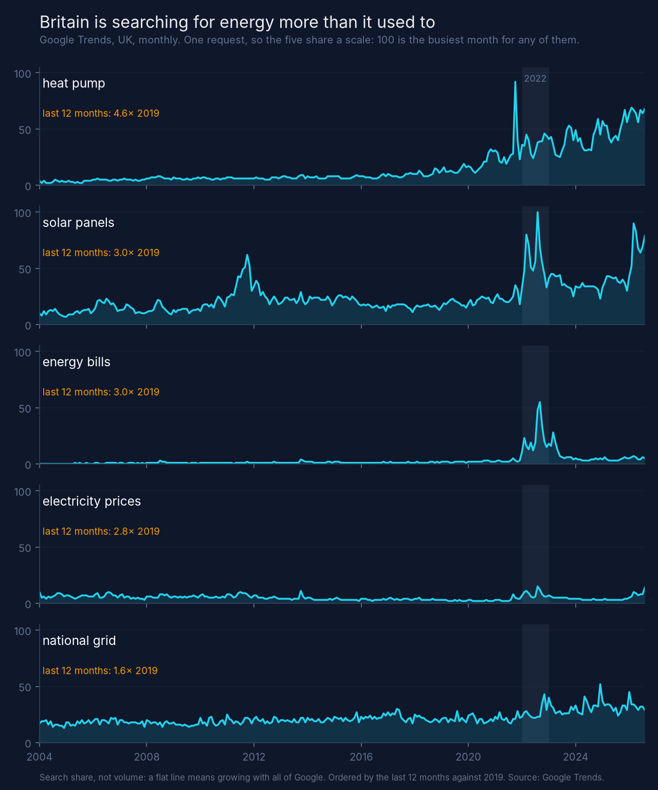
Interest in energy is not what it was. Measured by UK search interest against 2019, heat pumps are up 4.6 times and solar panels three times. Energy bills spiked in 2022 and settled at about three times their old level. The crisis put electricity on the front page, net zero made it political, and data centres made it a technology story.
So demand for the question rose just as the cost of answering it collapsed. The people newly interested — investors, civil servants, journalists, householders — are exactly the people who were never going to learn a proprietary modelling tool or read settlement files.
A worked example: rerunning a real day
I picked the tightest day of last winter. On 8 January 2025, GB wind fell from 15.6 GW to 1.6 GW and gas ran up from 4 GW to 18 GW.
The model covers 32 combined-cycle gas units, pumped storage, batteries and hydro. Every unit is either on or off, must respect its own minimum run and off times, and pays to start — the sort of yes/no problem that commercial solvers used to be bought for. The inputs are all free: notified output and declared limits from Elexon, demand from NESO, the gas price from National Gas (£42.04/MWh that day), and carbon at £52.54/t. It solves in about two seconds.
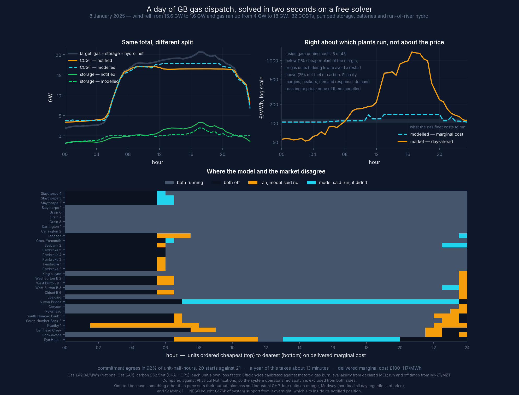
It gets the fleet right. The model agrees with what the plants actually notified in 92% of unit-half-hours, with 20 starts against 21. It is only moderately good on storage: the market ran pumped storage about eight times harder than a fuel-and-carbon objective can justify, because the market was also buying reserve, response and the option of a fast 1.7 GW.
The surprise was the outages. The two most efficient gas units in the fleet were unavailable all day, on the tightest day of the winter. Putting them back in the model saves about £415,000 in fuel, carbon and start-up costs, in a single day.
Why a gas plant can't just switch on
Most people picture a gas plant as a switch. It isn't, and the plants tell you so themselves: every unit declares its own limits to Elexon, publicly.
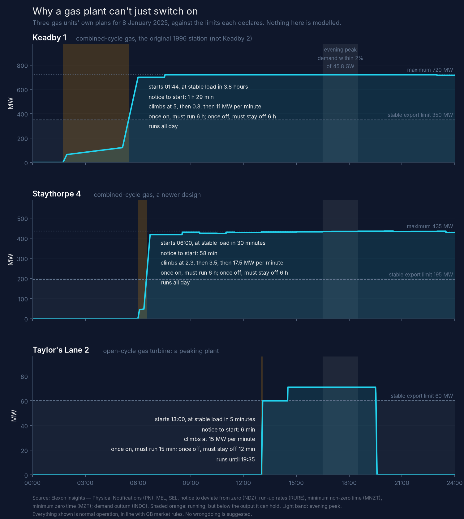
An older combined-cycle station started at 01:44 and took 3.8 hours to reach the lowest output it can hold steadily, creeping up at a declared 0.3 MW a minute through the middle of its warm-up. A newer one made it in 30 minutes. A small open-cycle turbine — a peaker — needed six minutes' notice and was at stable load five minutes after starting.
The times that follow matter more. Both combined-cycle units, once started, must run for six hours, and once stopped must stay off for six. The peaker's minimums are fifteen and twelve minutes. So having a big gas plant available for the evening peak means running it from the middle of the afternoon, whatever the price does in between. A peaker can wait.
That is also why peaking plant, batteries and demand response can set evening prices that the gas fleet cannot follow.
Nobody stops when it costs them money to stop
Look at the night before and the pattern is the same in reverse. Eleven gas units ran continuously from 18:00 on 7 January through to 06:00 on the 8th, and eight of them sat at exactly their minimum stable output all night. Between midnight and 6am the day-ahead price was £52–72/MWh. Their own running costs were £100–109. Against the day-ahead price, those six hours cost the fleet something like £890,000.
They did it because stopping means paying to restart, waiting out a minimum off time, and not being ready for the morning. Running at a loss overnight is cheaper than all three. (They earn elsewhere too — forward sales, reserve, balancing — so this is not a measure of profit.)
Where the model stops: the price
The model reproduces who runs. It does not reproduce what the electricity cost.
The market price sat inside the gas fleet's own running costs — £100–117/MWh — in only 8 of the day's 48 half-hours. It was above them in 25, averaging £569/MWh, and peaked at £1,353. The day averaged £336/MWh, and fuel and carbon for even the least efficient unit explain at most a third of that.
That gap is not evidence that gas was innocent. Gas plants may well have been setting the price, well above their running costs. On a day this tight, the explanations are some mixture of:
scarcity margin — a tight winter evening is when a plant earns one;
start-up costs and minimum run times priced in — a unit needed for two hours must recover a whole start and a six-hour run;
other providers at the margin — peakers, batteries, demand response, interconnectors, none of which are in my little stack;
and demand that responds to price, which a fixed demand target cannot represent at all.
A cost-minimising model with a fixed target can be accurate about which plants run, moderately good on storage, and still miss the price completely. That is worth knowing before you believe any model's price forecast, including the expensive ones.
Try it yourself
In the browser. model.energy is built by the people who maintain PyPSA and runs in a browser: pick a country, choose technologies, solve, and see the mix and the cost. No install, no Python.
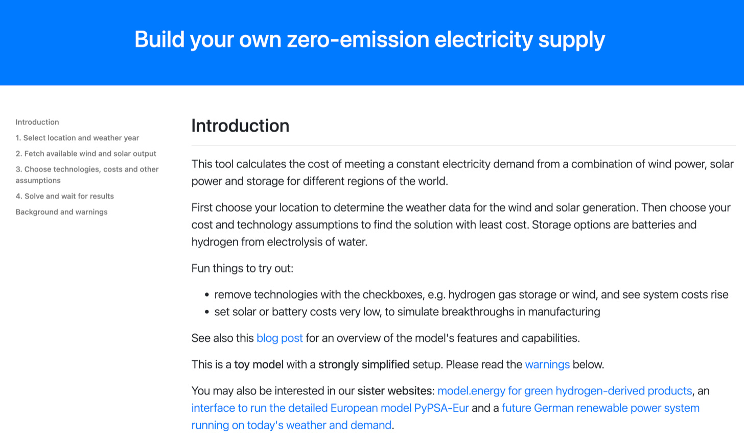
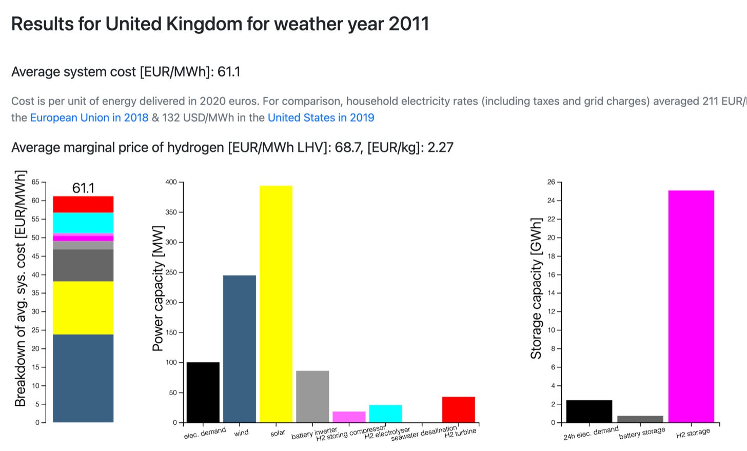
Ask it for a zero-emission supply for the United Kingdom and it comes back with a cost, a capacity mix and the storage needed to hold the thing together — in my run, €61/MWh on 2011 weather, with the wind, solar and hydrogen split laid out underneath. Its authors call it a toy model with a strongly simplified setup, and its numbers are not comparable with the model below — different demand, different technologies, different cost year. That is rather the point: you can disagree with it in about a minute.
In thirty lines. This builds ten British gas stations, with their real capacities and efficiencies, their declared minimum run times, and a start-up cost, then works out which run through a winter day — and what the electricity costs:
import pypsa

GAS, CARBON, CO2 = 42.04, 52.54, 0.184      # £/MWh gas, £/t carbon, t/MWh

n = pypsa.Network()
n.set_snapshots(range(24))
n.add("Bus", "GB")
n.add("Load", "demand", bus="GB", p_set=[d * 1000 for d in demand])
n.add("Generator", "wind", bus="GB", p_nom=20_000, p_max_pu=wind)
n.add("Generator", "nuclear", bus="GB", p_nom=6_500, marginal_cost=10)

for name, (mw, eff, stable, min_run) in ccgts.items():
    n.add("Generator", name, bus="GB", p_nom=mw, efficiency=eff,
          marginal_cost=(GAS + CARBON * CO2) / eff,
          committable=True,          # on or off: a yes/no decision
          p_min_pu=stable,           # can't run below this once on
          min_up_time=min_run,       # once started, must stay on
          start_up_cost=40 * mw, up_time_before=0)

n.optimize()
It prints which stations run in which hour:
hour           012345678901234567890123
Keadby 2       ······■■■■■■■■■■■■■■■■■■
Staythorpe     ······■■■■■■■■■■■■■■■■■■
Grain          ·······■■■■■■■■■■■■■■■■■
Pembroke       ········■■■■■■■■■■■■■■■·
Didcot B       ·············■■■■■■■····
Sutton Bridge  ················■■■■■···
an older CCGT  ···············■■■■■■···
Three things fall out of it. Nobody told it to start the most efficient station first; that is just what costs least. The plants needed only for the 5pm peak run from 3pm to 9pm, because their minimum run time says so. And the price at 5pm is £191/MWh when the marginal plant costs £117/MWh to run: the difference is the cost of starting a plant for a short peak, spread into the price. The argument three sections up, in miniature.
Where to run it. A laptop is fine: the example above solves in under a second, the January day in about two, a year of it in about thirteen minutes. For bigger work — all of Europe, many years, many scenarios — it is straightforward to run on a rented server or a shared notebook environment instead of buying a powerful desktop. The course itself ran that way, with everyone working in a browser.
Properly. The documentation and the code are open, the Birmingham course materials are published under a Creative Commons licence, and PyPSA Labs run the training.
I went to Birmingham expecting to learn a modelling tool and came back with a different thought. The data has been free for twenty years. The software is now free too, and fast enough to answer a serious question on a laptop over a coffee. What is left is knowing which question to ask, and whether the answer that comes back is any good.
Next: I stopped telling the model what exists, and asked it where it would build Britain's wind and solar instead. The answer is not where we put them.
Thanks to PyPSA Labs and the Supergen Energy Networks Hub, who ran and hosted the course, and to the University of Birmingham.